Tuesday, December 6, 2016

Get Keras ready with Theano backend

Keras is a deep learning library for Theano and TensorFlow which is written in Python. It allows you to build deep learning models with a few code lines. And also it enables fast experimentation. It is compatible with Python 2.7-3.5.

The name Keras was based on a Greek mythology. Keras means 'Horn' in Greek. They believed that the dream spirits who come through the polished horn, have truth behind them. Keras was initially build as a part of the research project, ONEIROS (Open-ended Neuro-Electronic Intelligent Robot Operating System)

Keras library has following characteristics

  • Easy and fast prototyping
  • Supports both convolutional networks and recurrent networks.
  • Supports arbitrary connectivity schemes
  • Run flawlessly on CPU and GPU

There are four guiding principles for Keras

  1. Modularity- A model is understood as a sequence or a graph of standalone, fully-configurable modules that can be plugged together with as little restrictions as possible. In particular, neural layers, cost functions, optimizers, initialization schemes, activation functions, regularization schemes are all standalone modules that you can combine to create new models.
  2. Minimalism-Each module should be kept short and simple. Every piece of code should be transparent upon first reading. No black magic: it hurts iteration speed and ability to innovate.
  3. Easy extensibility- New modules are dead simple to add (as new classes and functions), and existing modules provide ample examples. To be able to easily create new modules allows for total expressiveness, making Keras suitable for advanced research.
  4. Work with Pyhton-No separate models configuration files in a declarative format. Models are described in Python code, which is compact, easier to debug, and allows for ease of extensibility.

Theano


Theano is a mathematical symbolic expression compiler. It's tightly integrated with Python ecosystem. It can use GPUs and perform efficient symbolic differentiation. This was designed to handle the complex computations of Deep learning. It handles multidimensional arrays like Numpy. There are many opensource deep learning libraries built on top of Theano, like Keras. Google created Tensorflow to replace Theano. However there is no huge difference  between Theano and TensorFlow. 

To install Theano and Keras, refer the Keras documentation here. If you are using Windows 10, refer this article here.

Note: There is no point of installing CUDA , if you don't have NVidia graphical processing unit. Then  Theano will run on CPU instead of GPU. If you have NVidia card, I highly recommend you to install CUDA, the performance will be high when Theano runs on GPU.  


Friday, December 2, 2016

Let's build a Neural Network with a few lines of code CONTINUED

Before we go deeper into Neural networks, I thought it would be better if we could learn how to predict output values for new inputs through a trained neural network. You need to do a small change to the previous code. This is assuming that the current neural network is fully optimized. In this example I'm not going to re-train the network with the new input, I'm just using the updated weights.

  1. import numpy as la
  2. from xlwings import xrange
  3. # input data
  4. X1 = la.array([[0, 0, 1], [1, 0, 1], [0, 1, 1]])
  5. # output data
  6. X2 = la.array([[0, 1, 0]]).T
  7. # new input
  8. X3 = la.array([1, 1, 1])  
  9. # sigmoid function
  10. def sigmoid(x, derivative=False):
  11.     if (derivative == True):
  12.         return x * (1 - x)
  13.     return 1 / (1 + la.exp(-x))
  14. # Generate random numbers
  15. la.random.seed(1)
  16. # initialize weights with mean 0
  17. synapse0 = 2 * la.random.random((3, 1)) - 1
  18. for iterations in xrange(10000):
  19.     # forward propagation
  20.     layer0 = X1
  21.     layer1 = sigmoid(la.dot(layer0, synapse0))
  22.     # error calculation
  23.     layer1_error = X2 - layer1
  24.     # multiply slopes by the error
  25.     # (reduce the error of high confidence predictions)
  26.     layer1_delta = layer1_error * sigmoid(layer1, True)
  27.     # weight update
  28.     synapse0 += la.dot(layer0.T, layer1_delta)
  29. #output for new input data
  30. predictedOutput = sigmoid(la.dot(X3, synapse0)
  31. print("Trained output:")
  32. print(layer1)
  33. print("Output for the new input:"
  34. print(predictedOutput)

The new output will be as follows;

Trained output:
[[ 0.01225605]
 [ 0.98980175]
 [ 0.0024512 ]]
Output for the new input:
[ 0.9505469]


Our new input row is highlighted in the below table.


Input
Output
0
0
1
0
1
0
1
1
0
1
1
0
1
1
1
1


9. X3 = la.array([111])  

With this line, we assign the new input to X3. 


39predictedOutput= sigmoid(la.dot(X3, synapse0)


With this line, we multiply the new input by the updated weights. The network is already optimized to the given input. Therefore neural network  can just apply the finalized weights to the new input. 


By adding the following code line, after the 'for loop',  you can see the updated weights.

print(synapse0)


If  we don't train the network further, for more data, the same updated weights will be applied to new data and predict the output value.

You can now check the output by reducing the number of iterations drastically. The value of updated weights will be different and the error will be quite high. There is no optimal number of iterations. However you should iterate the training until there is no significant decrease in error.

If you have any issues or questions with this post, please feel free to contact me at any time. 😊


Thursday, December 1, 2016

Let's build a Neural Network with a few lines of code

In my previous post, I mentioned how to setup Python. Today I'm going to build a simple 2 Layer neural network using backpropagation. Let's start with the code. I prefer to understand the code before going for complicated theories and concepts. Because the other way round doesn't work for me. 😄


  1. import numpy as la
  2. from xlwings import xrange
  3. # input data
  4. X1 = la.array([[0, 0, 1], [1, 0, 1], [0, 1, 1]])
  5. # output data
  6. X2 = la.array([[0, 1, 0]]).T
  7. # sigmoid function
  8. def sigmoid(x, derivative=False):
  9.     if (derivative == True):
  10.         return x * (1 - x)
  11.     return 1 / (1 + la.exp(-x))
  12. # Generate random numbers
  13. la.random.seed(1)
  14. # initialize weights with mean 0
  15. synapse0 = 2 * la.random.random((3, 1)) - 1
  16. for iterations in xrange(10000):
  17.     # forward propagation
  18.     layer0 = X1
  19.     layer1 = sigmoid(la.dot(layer0, synapse0))
  20.     # error calculation
  21.     layer1_error = X2 - layer1
  22.     # multiply slopes by the error
  23.     # (reduce the error of high confidence predictions)
  24.     layer1_delta = layer1_error * sigmoid(layer1, True)
  25.     # weight update
  26.     synapse0 += la.dot(layer0.T, layer1_delta)
  27. print("Trained output:")
  28. print(layer1)

The above code will give the below output.


Trained output:
[[ 0.01225605]
 [ 0.98980175]
 [ 0.0024512 ]]


The following table contains the input dataset and output dataset which the neural network was based on. As you can see, the highlighted input column is correlated with the output column. What we are trying to do here is, create a model to predict the output with the given input.


Input
Output
0
0
1
0
1
0
1
1
0
1
1
0


We can see the following characteristics when building a neural network using backpropagation.
  • Assign random weights while initializing the network
  • Provide input data to the network and calculate the output
  • Compute the error by comparing the network output and correct output(error function) 
  • Propagate the error term back to the previous layer and update the weights and then repeat this until the error stops improving

Let's try to understand the code.

1. import numpy as la


Numpy is a scientific computing library in Python. It contains useful linear algebra, Fourier transform, N-dimensional array objects etc. In this example, we use it for arrays and random number generations.


5. X1 = la.array([[001][101][011]])


6. X2 = la.array([[010]]).T

In lines 5&6, we assign the arrays of input and output to X1 and X2 respectively. We take transpose (T) of the output dataset to match with the input. Because input is a 3x3 matrix and we need to obtain the 3x1 matrix of output.


10. def sigmoid(x, derivative=False):
11.    if (derivative == True):
12.        return x * (1 - x)
14.    return 1 / (1 + la.exp(-x))


In backpropagation we need proper activation function to activate the hidden unit. The activation function should be continuous, easy to compute, non decreasing and non differential.  Sigmoid function satisfies almost all the conditions. Sigmoid function go either from 0 to 1 or from -1 to 1 based on the convention. In here, we use values between 0 and 1 for converting numbers to probabilities.
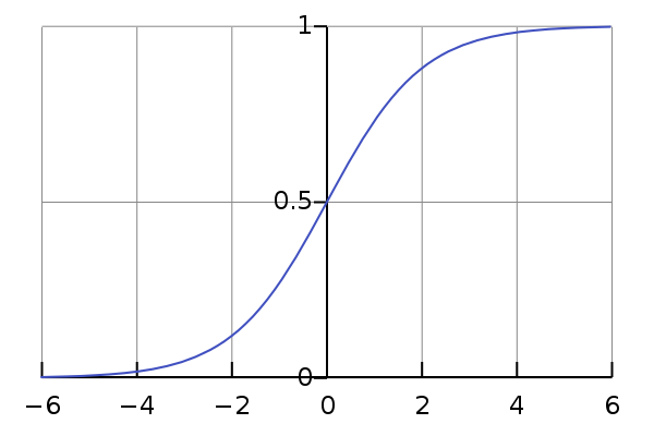


We use the first derivative of the Sigmoid function to calculate the gradient since it is very convenient. If you are not good with derivatives, refer tutorials. 


16. la.random.seed(1)

This line generates random numbers for the calculation.


19. synapse0 = 2 * la.random.random((31)) - 1

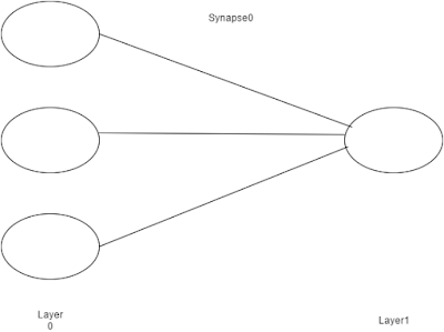
In real world, synapse assist in passing electrical or chemical signal between the neurons. There is no much difference in machine learning, we use synapse as a matrix of weights to connect input layer with the output layer. In this scenario we have only two layers therefore we need only one matrix of weights. It's a 3x1 matrix since we have three inputs and one output.


In this line, weights will be initialized with mean zero. Because initially system is unsure of the weights. However as the system learns, it becomes sure of it's output probabilities.


21. for iterations in xrange(10000):

In our code, training starts from here. The xrange() function generates list of integers. This loop iterates for several times to optimize our network to the given datasets.


24. layer1 = sigmoid(la.dot(layer0, synapse0))

In this step the network predict output for the given input. The synapse0 matrix will be multiplied by the layer0 matrix and will be sent to the Sigmoid function.


Then the network will provide 3 output guesses for the given input.


27. layer1_error = X2 - layer1

In this line, it calculates how much the guessed output deviated from the correct output.


31. layer1_delta = layer1_error * sigmoid(layer1, True)


This is the most important code line. If we reconsider the Sigmoid diagram, you can see that it has shallow slope when it comes to high positive/negative values. And the steepest slope will be at zero. If the network guessed high positive/negative values for some output that means it is quite confident about the result. Therefore those values will be multiplied by the values which are closer to zero in order to reduce the effect. And if  some values are closer to zero, it means that network is not much confident about these values. Then those values should be heavily updated.


The network use the three input training sets at the same time which is called "full batch configuration". However to explain the scenario I'll use just one training example.


In this instance, the top weight will be updated slightly. It is because the network is already confident with the value.


You can debug the code and check how this really works, it's quite amazing. 😊
Now you can check the result for simple AND truth table and think why you got such a result.
Hope to go deeper into the neural networks with my next post. Let's see 😜